Campus Recruitment

Campus recruitment is a strategy for sourcing, engaging and hiring young talent for internship and entry-level positions. College recruiting is typically a tactic for medium- to large-sized companies with high-volume recruiting needs, but can range from small efforts (like working with university career centers to source potential candidates) to large-scale operations (like visiting a wide array of colleges and attending recruiting events throughout the spring and fall semester). Campus recruitment often involves working with university career services centers and attending career fairs to meet in-person with college students and recent graduates.
Our dataset revolves around the placement season of a Business School in India. Where it has various factors on candidates getting hired such as work experience,exam percentage etc., Finally it contains the status of recruitment and remuneration details.
There are 3 primary goal in this project, first do a exploratory analysis of the Recruitment dataset, second do an visualization analysis of the Recruitment dataset and last predict whether a student got placed or not using classification models.
Data Fields
Import Package and Data
import pandas as pd
import numpy as np
import matplotlib.pyplot as plt
import seaborn as sns
import sklearn
%matplotlib inline
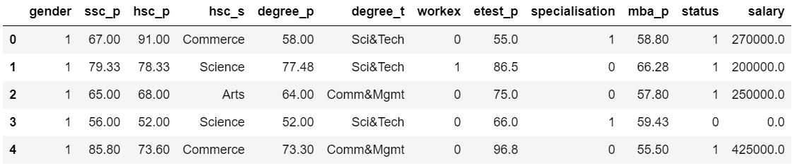
For this exercise, the data set (.csv format) is uploaded to my repository github, read into the Jupyter notebook and stored in a Pandas DataFrame.
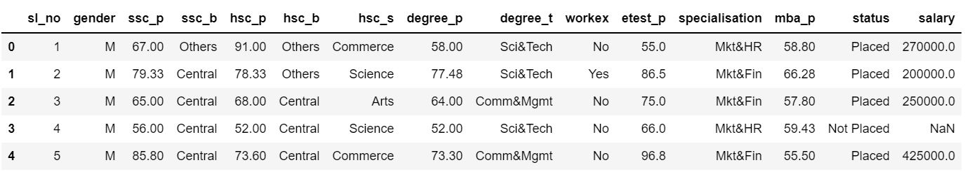
We have Gender and Educational qualification data. We have all the educational performance(score) data. We have the status of placement and salary details. We can expect null values in salary as candidates who weren't placed would have no salary. Status of placement is our target variable rest of them are independent variable except salary.
Data Preparation and Cleaning
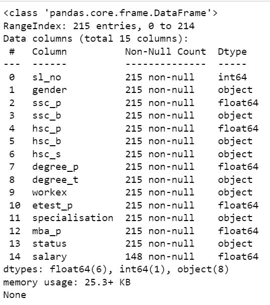
We have 215 candidate details and there are mixed datatypes in each column. We have few missing values in the salary column as expected since those are the people who didn't get hired. We also have 1 integer,5 float and 8 object datatypes in our dataset
Checking Missing Value
Datasets in the real world are often messy, However, this dataset is almost clean and simple. But lets check the missing value first
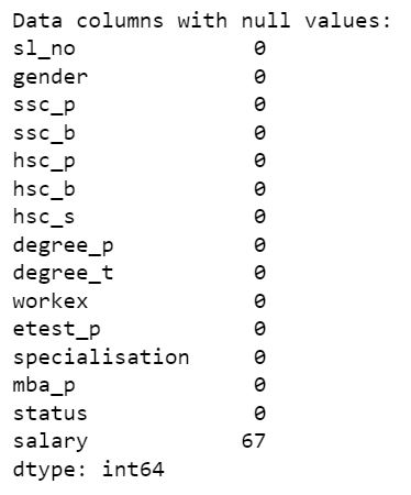
There are 67 null values in our data, which means 67 unhired candidates. We can't drop these values as this will provide a valuable information on why candidates failed to get hired. We can't impute it with mean/median values and it will go against the context of this dataset and it will show unhired candidates got salary. Our best way to deal with these null values is to impute it with '0' which shows they don't have any income.
Handling Missing Value
First lets focus on the missing data in review features,if we drop the rows which has null values we might sabotage some potential information from the dataset. So we have to impute values into the NaN records which leads us to accurate models. Since it is a salary feature,it is best to impute the records with '0' for unhired candidates
After we replace missing value with '0' now we need to drop unwanted features. We have dropped serial number as we have index as default and we have dropped the boards of school education as I believe it doesn't matter for recruitment.
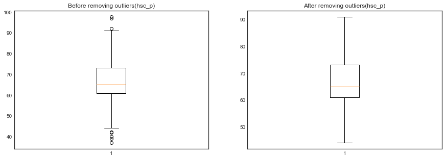
Outliers
Outliers are unusual values in your dataset, and they can distort statistical analyses and violate their assumptions. Unfortunately, all analysts will confront outliers and be forced to make decisions about what to do with them. Given the problems they can cause, you might think that it’s best to remove them from your data. But, that’s not always the case. Removing outliers is legitimate only for specific reasons.Outliers can be very informative about the subject-area and data collection process. It’s essential to understand how outliers occur and whether they might happen again as a normal part of the process or study area. Unfortunately, resisting the temptation to remove outliers inappropriately can be difficult. Outliers increase the variability in your data, which decreases statistical power. Consequently, excluding outliers can cause your results to become statistically significant. In our case, let's first visualize our data and decide on what to do with the outliers.
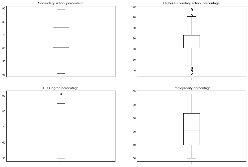
As you see, we have very less number of outliers in our features. Especially we have majority of the outliers in hsc percentage. lets see the visualize after removing outliers.
Exploratory Data Analysis
Count of categorical features- Count plot
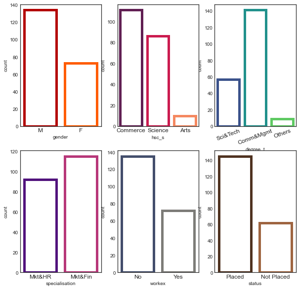
From the visualize we can see that We have more male candidates than female, We have candidates who did commerce as their hsc course and as well as undergrad, Science background candidates are the second highest in both the cases, Candidates from Marketing and Finance dual specialization are high, Most of our candidates from our dataset don't have any work experience and most of our candidates from our dataset got placed in a company.
Distribution Salary- Placed Students
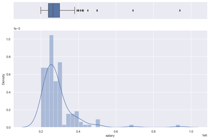
Many candidates who got placed received package between 2L-4L PA. Only one candidate got around 10L PA and the average of the salary is a little more than 2LPA.
Employability score vs Salary- Joint plot
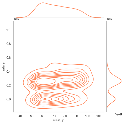
Most of the candidates scored around 60 percentage got a decent package of around 3 lakhs PA. Not many candidates received salary more than 4 lakhs PA and The bottom dense part shows the candidates who were not placed.
Distribution of all percentages
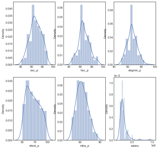
All the distributions follow normal distribution except salary feature. Most of the candidates educational performances are between 60-80%. Salary distribution got outliers where few have got salary of 7.5L and 10L PA
Work experience Vs Placement Status
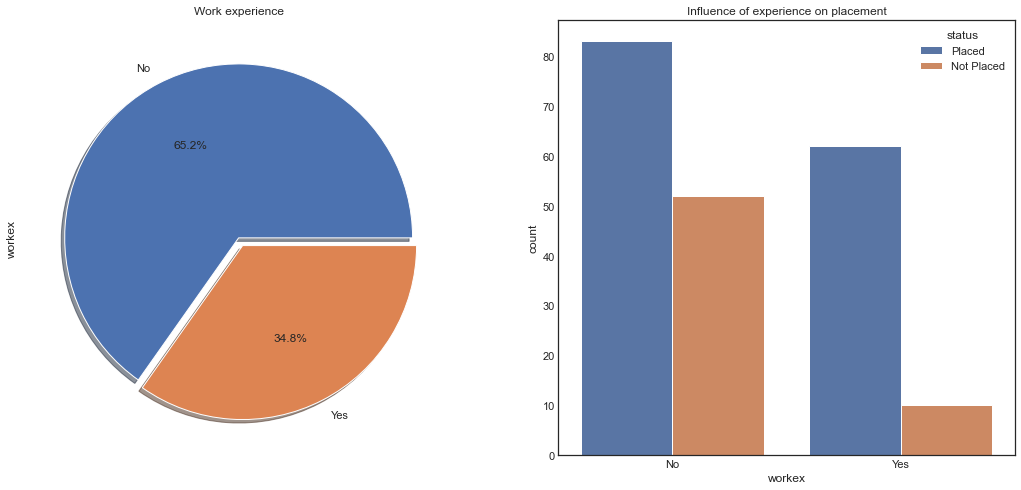
We have nearly 66.2% of candidates who never had any work experience. Candidates who never had work experience have got hired more than the ones who had experience. We can conclude that work experience doesn't influence a candidate in the recruitment process.
MBA marks vs Placement Status- Does your academic score influence?
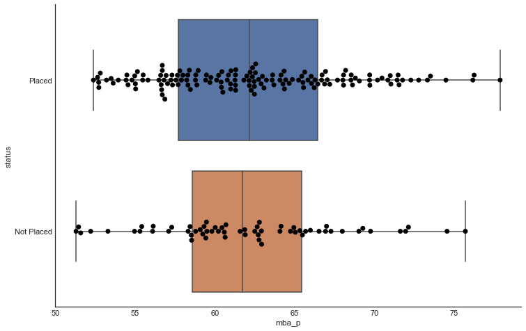
Comparitively there's a slight difference between the percentage scores between both the groups, But still placed candidates still has an upper hand when it comes to numbers as you can see in the swarm. So as per the plot,percentage do influence the placement status
Does MBA percentage and Employability score correlate?
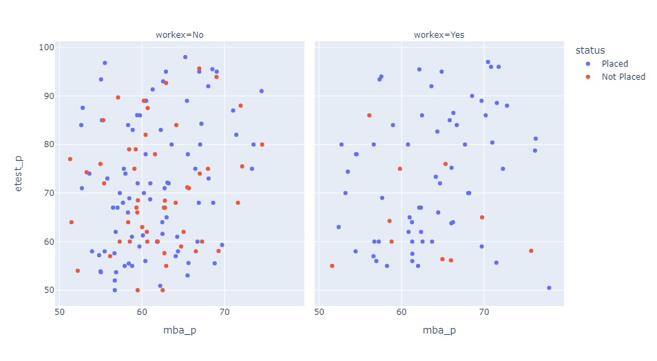
There is no relation between mba percentage and employability test. There are many candidates who haven't got placed when they don't have work experience and most of the candidates who performed better in both tests have got placed.
Is there any gender bias while offering remuneration?
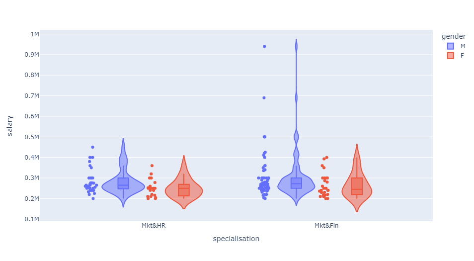
The top salaries were given to male. The average salary offered were also higher for male. More male candidates were placed compared to female candidates.
Coorelation between academic percentages
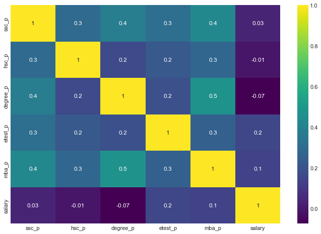
Candidates who were good in their academics performed well throughout school,undergrad,mba and even employability test. These percentages don't have any influence over their salary.
Distribution of our data
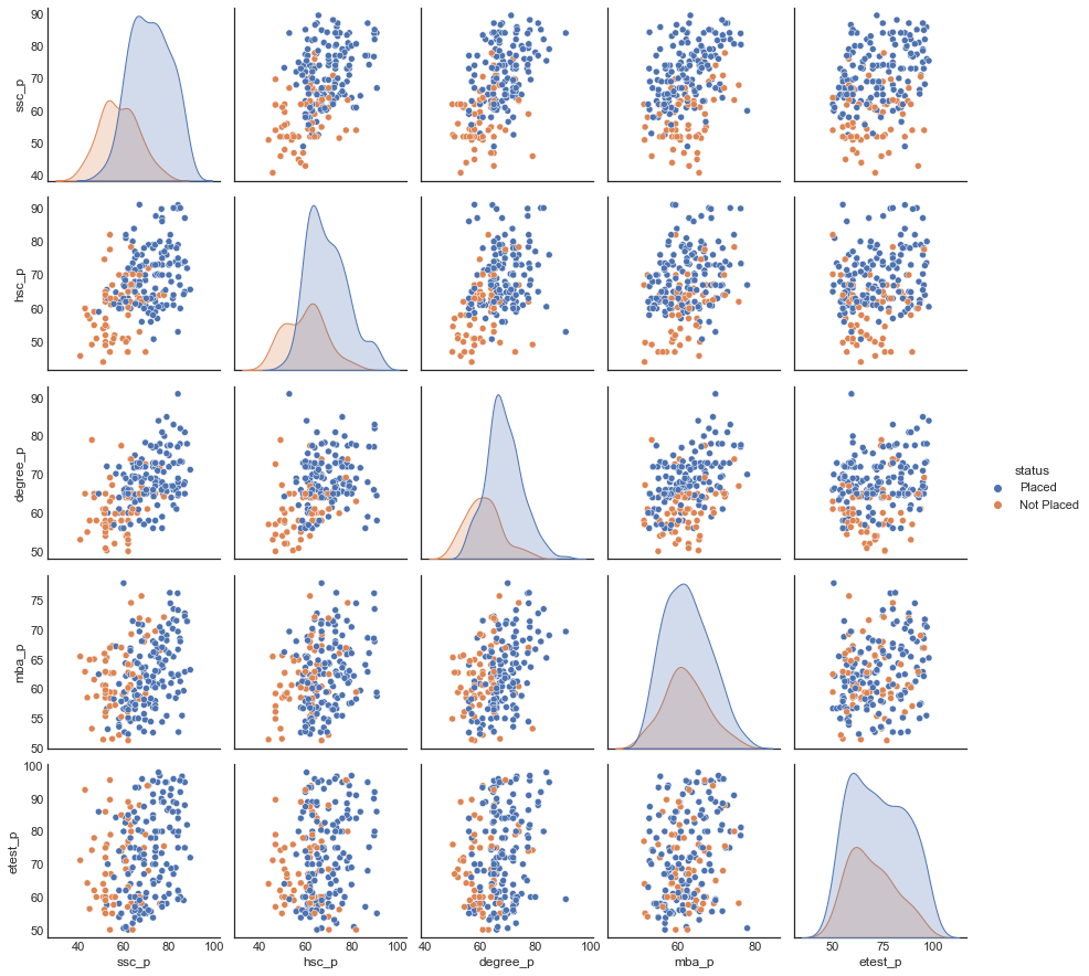
Candidates who has high score in higher secondary and undergrad got placed. Whomever got high scores in their schools got placed. Comparing the number of students who got placed candidates who got good mba percentage and employability percentage.
Data Preprocessing
Now let's welcome our data to the model.Before jumping onto creating models we have to prepare our dataset for the models. We dont have to perform imputation as we dont have any missing values but we have categorical variables which needs to be encoded.
Label Encoding
We have used label encoder function for the category which has only two types of classes.
One hot encoding
We have used dummies function for the category which has more than two types of classes
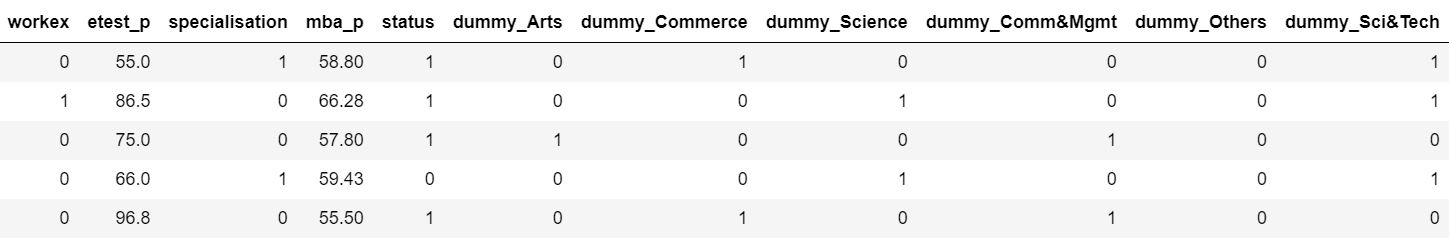
Assigning the target(y) and predictor variable(X)
Our Target is to find whether the candidate is placed or not. We use rest of the features except 'salary' as this won't contribute in prediction(i.e) In real world scenario, students gets salary after they get placed, so we can't use a future feature to predict something which happens in the present
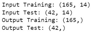
Train and Test Split (80:20)
Next we split the dataset into train and test in 80:20.
Machine Learning Models
Now let's feed the models with our data Objective: To predict whether a student got placed or not
Logistic Regression
Let's fit the model in logistic regression and figure out the accuracy of our model

Confusion Matrix and Classification Report
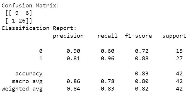
The Confusion matrix result is telling us that we have 9+26 correct predictions and 1+6 incorrect predictions. The Classification report reveals that we have 84% precision which means the accuracy that the model classifier not to label an instance positive that is actually negative and it is important to consider precision value because when you are hiring, you want to avoid Type I errors at all cost. They are culture killers. In hiring, a false positive is when you THINK an employee is a good fit, but in actuality they’re not.
ROC Curve
Let's check out the performance of our model through ROC curve
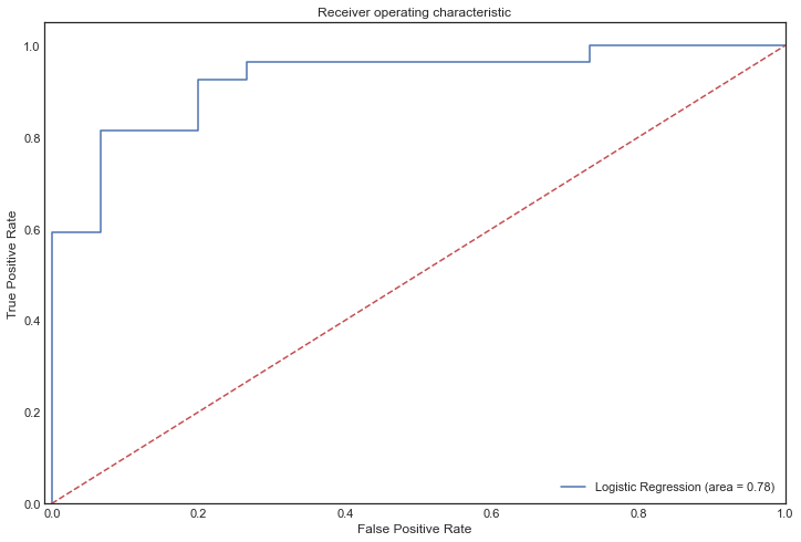
From the ROC curve we can infer that our logistic model has classified the placed students correctly rather than predicting false positive. The more the ROC curve(blue) lies towards the top left side the better our model is. We can choose 0.8 or 0.9 for the threshold value which can reap us true positive results
Random Forest
lets use random forest to create a aggregation of trees and produce accurate results and we have an accuracy of 76%
Looking at Feature Importance
Let's see which feature influences more on making the decision and we should cut it off to make our model accurate
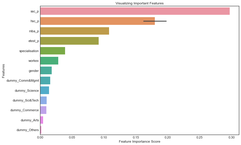
As we see the school and undergrad specialisations have less influence in classifying the model. But it is really wierd to acknowledge ssc_p influencing more in classifying
Pruning out less important feature
Let's cut off the less important feature and check for model accuracy.
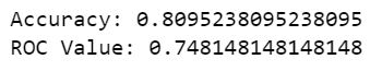
Great. Now We have an accuracy of 81% and the ROC value 75% indicates the models have classified better without having much false positive predictions
K Nearest Neighbours
Let's try out a lazy supervised classification algorithm. Our beloved, KNN
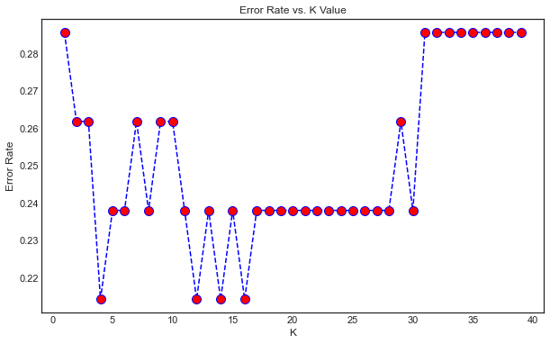
There are a lot of ups and downs in our graph. If we consider any value between 10-15 we may get an overfitted model. So let's stick onto the first trough. Our K value is 5
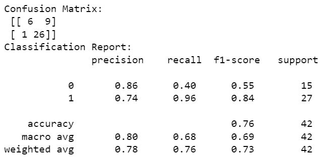
Our model has precisely classified 86% of Not placed categories and 74% of Placed categories. To talk in numbers 26+6 correct classifications and 1+9 false negative and false positive classification. We should be considering the precision value as our metric because the possibility of commiting False Positive is very crucial in recuritment
Naive Bayes Classifier with Cross Validation
Let's use Naive Bayes model for our dataset. Since our outcome feature has 1,0(placed, not placed) we can go with Bernoulli Naive bayes algorithm and also let's measure the accuracy with cross validation

Our cross validation precision is approximately 73.5%
Support Vector Machine
Let's use SVM to classify our output feature
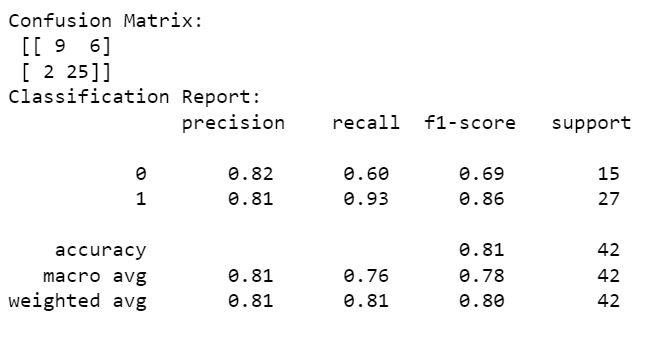
We have got 82% and 81% precision in classifying our model. 9+25 correctly classified and 2+6 wrongly classified( False Negative & False Positive)
XGBoost
Let's try our the state of art ensemble model XGBoost. We have used RMSE metrics for model performance
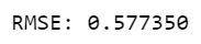
The error value of our model is just 0.577. Now let's use cross validation and try to minimise further.
XGBoost with Cross Validation
In this algorithm we are using DMatrix to convert our dataset into a matrix and produce the output in dataframe.
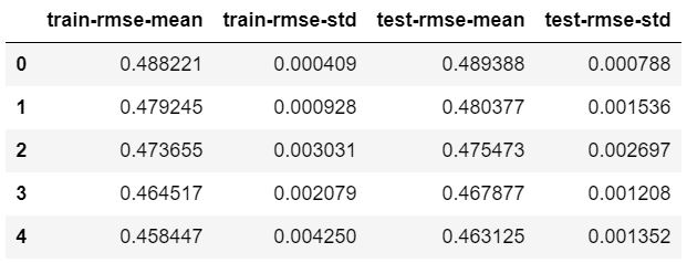
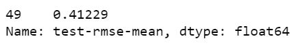
We have reduced our model error to 0.41.
Summary
From the analysis report on Campus Recruitment dataset here are my following conclusions: