Exploratory Data Analysis
Ames House

The Ames housing data set (De Cock 2011) is an excellent resource for learning about models that we will use throughout this project. It contains data on 2,930 properties in Ames, Iowa, including columns related to house characteristics, location, lot information, rating of condition and quality and saleprice. Arie will provide details about EDA, and make insight from data visualize using R Programming Language.
Data Fields
Import Package and Data
Started with imports of some basic libraries that are needed throughout the case. This includes dplyr, tidyr, stringr, lubridate. For visualization we use ggplot2 and plotly.
library(dplyr)
library(tidyr)
library(stringr)
library(lubridate)
library(ggplot2)
library(plotly)
For this exercise, the data set (.csv format) is downloaded to a local folder.
df <- read.csv('House Price.csv')
Start With the Target
Perform a univariate analysis of the target variable, namely SalePrice and describe what insights can be obtained.
##find missing value:
df %>% is.na() %>% colSums()
#no missing value in SalePrice
##check mean, mode, Min Value, Max Value, and Standard Deviation
getmode <- function(v) {
uniqv <- unique(v)
uniqv[which.max(tabulate(match(v, uniqv)))]
}
getmode(df$SalePrice) #mode
sd(df$SalePrice) #SD
summary(df$SalePrice) #min, max, median
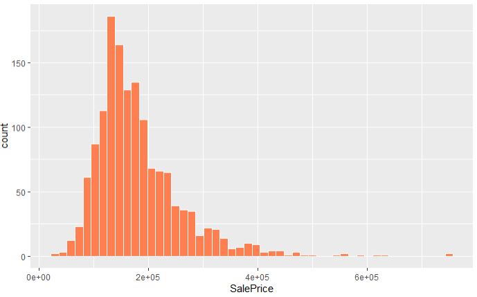
ggplot(data = df, mapping = aes(x = SalePrice)) +
geom_histogram(bins = 50, color = "white", fill = "coral") #Visualize histogram SalePrice
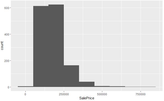
ggplot(df, aes(SalePrice)) +
geom_histogram(binwidth = 100000) #Visualize histogram with binwidth 100000
We can look visualize histogram with binwidth 100000.
Insight
- From the histogram display, it can be concluded that the sale price data is not normally distributed and tends to be skewed to the left.
- the most sold house with a price of 140000.
- The most expensive house is sold for 755000 which is an outlier from the data.
- Saleprice house data is distributed under the price of 250000.
Find the 5 variables with the strongest correlation (positively or negatively) with SalePrice
cor.test(df$MSSubClass,df$SalePrice) # -0.084
cor.test(df$LotFrontage,df$SalePrice) # 0.35
cor.test(df$LotArea,df$SalePrice) # 0.26
cor.test(df$OverallQual,df$SalePrice) # 0.790
cor.test(df$OverallCond,df$SalePrice) # -0.077
cor.test(df$YearBuilt,df$SalePrice) # 0.522
cor.test(df$YearRemodAdd,df$SalePrice) # 0.507
cor.test(df$MasVnrArea,df$SalePrice) # 0.477
cor.test(df$BsmtFinSF1,df$SalePrice) # 0.386
cor.test(df$BsmtFinSF2,df$SalePrice) # -0.011
cor.test(df$BsmtUnfSF,df$SalePrice) # 0.214
cor.test(df$TotalBsmtSF,df$SalePrice) # 0.613
cor.test(df$X1stFlrSF,df$SalePrice) # 0.605
cor.test(df$X2ndFlrSF,df$SalePrice) # 0.319
cor.test(df$LowQualFinSF,df$SalePrice) # -0.0256
cor.test(df$GrLivArea,df$SalePrice) # 0.708
cor.test(df$BsmtFullBath,df$SalePrice)# 0.227
cor.test(df$BsmtHalfBath,df$SalePrice) # -0.0168
cor.test(df$BedroomAbvGr,df$SalePrice) # 0.168
cor.test(df$KitchenAbvGr,df$SalePrice) # -0.135
cor.test(df$TotRmsAbvGrd,df$SalePrice) # 0.533
cor.test(df$Fireplaces,df$SalePrice) # 0.466
cor.test(df$GarageYrBlt,df$SalePrice) # 0.486
cor.test(df$GarageCars,df$SalePrice) # 0.640
cor.test(df$GarageArea,df$SalePrice) # 0.623
cor.test(df$WoodDeckSF,df$SalePrice) # 0.324
cor.test(df$OpenPorchSF,df$SalePrice) # 0.315
cor.test(df$EnclosedPorch,df$SalePrice) # -0.128
cor.test(df$X3SsnPorch,df$SalePrice) # 0.044
cor.test(df$ScreenPorch,df$SalePrice) # 0.111
cor.test(df$PoolArea,df$SalePrice) # 0.0924
cor.test(df$MiscVal,df$SalePrice) # -0.0211
cor.test(df$MoSold,df$SalePrice) # 0.0464
cor.test(df$YrSold,df$SalePrice) # -0.0289
Insight
POSITIVE STRONG CORRELATION
- OverallQual : this makes sense if the higher the SalePrice, the quality of the house can be said to be better from the range 1-10.
- GrLivArea : this makes sense if the higher the SalePrice of a house, the house will have a large living room size too.
- GarageCars : this makes sense if the higher the SalePrice the house will have a garage that can fit a few more cars than the cheaper house.
- GarageArea : this makes sense because a house with a high sale price will have a high garage area too.
- TotalBsmtSF : this makes sense because houses with high sales prices have a large basement too.
NEGATIVE STRONG CORRELATION
- EnclosedPorch : Saleprice is weakly negatively correlated with the enclosed patio area so it can be ignored and this doesn't make sense because neither houses with low salesprice nor high average have a covered terrace.
- KitchenAbvGr : SalePrice has a weak negative correlation with KitchenAbvGr so it can be ignored and this can be said to be unreasonable/does not affect SalePrice because the average house has 1 kitchen, either cheap or expensive.
- LowQualFinSF : SalePrice has a weak negative correlation with LowQualFinSF and this can be said to be reasonable because the higher the price, the lower the floor area of low quality, but this can also be ignored because the correlation is low.
- MSSubClass : Saleprice has a weak negative correlation with MSSubClass so this can be ignored and this also doesn't make sense because every number from MSSubClass is categorical data where the highest SalePrice is in categorical 60 which is a new house with 2 floors.
- OverallCond : SalePrice has a weak negative correlation with OverallCond so this can be ignored and this doesn't make sense because the highest and lowest salesprice are in the same OverallCond value of 5.
It is never hurt to test basic knowledge
There is a view that a low OverallQual has a lower price tendency, and a house with a higher OverallQual Quality has a higher price tendency. Perform an analysis of the relationship between OverallQual and SalePrice.
df %>% ggplot(aes(x=OverallQual,y=SalePrice)) + geom_point()
cor.test(df$OverallQual,df$SalePrice)
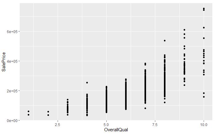
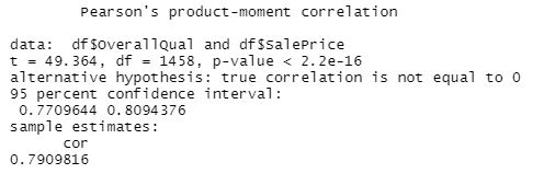
Insight
OverallQual can be said to be a categorical variable which is described in numerical form 1-10, where 1 is very bad and 10 is very good. a high price has a high OverallQual. Based on the correlation, it can be seen that SalePrice and OverallQUall have a very strong correlation, namely 0.790 and it can be concluded that OverallQual greatly affects SalePrice from home.
Beware of False Correlation
There is a tendency that new homes have a higher price. However, we should not be in a hurry to conclude that a new house must have a higher selling price, because if the new house that is built is not good, of course the price cannot be high either. What do you think makes a new home a higher value?
df %>% ggplot(aes(x=YearBuilt,y=YearRemodAdd)) + geom_point()
df %>%
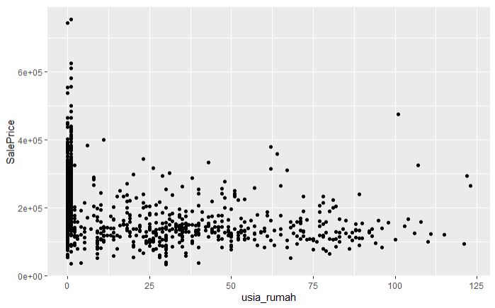
mutate(df, usia_rumah = YearRemodAdd-YearBuilt, .after ="SalePrice" ) %>%
ggplot(aes(x=usia_rumah,y=SalePrice)) + geom_point()
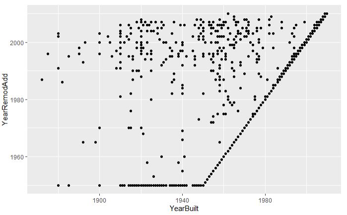
Insight
The thing that makes new homes have a higher value is when they do YearRemodadd with a short period of time with YearBuilt. Through visualization, it can be seen that houses that were carried out YearRemodadd and YearBuilt in the same year tend to have a higher sale price.
Haunted places(?)
Pay attention to the following scatter plot
df %>% ggplot(aes(x=GrLivArea,y=SalePrice)) + geom_point()
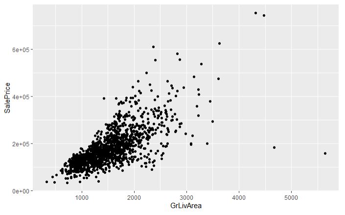
On the right, there are two houses, which have a very large GreenLivingArea, but the SalePrice is cheap. Lets analyze why the two houses are cheap.
df %>% ggplot(aes(x=GrLivArea,y=SalePrice)) +
  geom_point()+
  coord_cartesian(xlim=c(4500,6000)) #visualize house with GrLivArea >4500
x<- filter(df, GrLivArea>4500) #filter house with GrLivArea diatas 4500
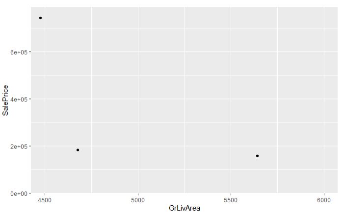
Insight
The two houses cheap robably because even though the house has a large GrLvArea area, the house is on a bad contour where its position is at a sharp turn and on an incline. houses with LandCountour type 'Bnk' do not have a high selling value.
EDA for Top Month Sold
df %>% ggplot(aes(x=YearBuilt,y=YearRemodAdd)) + geom_point()

df %>%
  mutate(df, usia_rumah = YearRemodAdd-YearBuilt, .after ="SalePrice" ) %>%
  ggplot(aes(x=usia_rumah,y=SalePrice)) + geom_point()
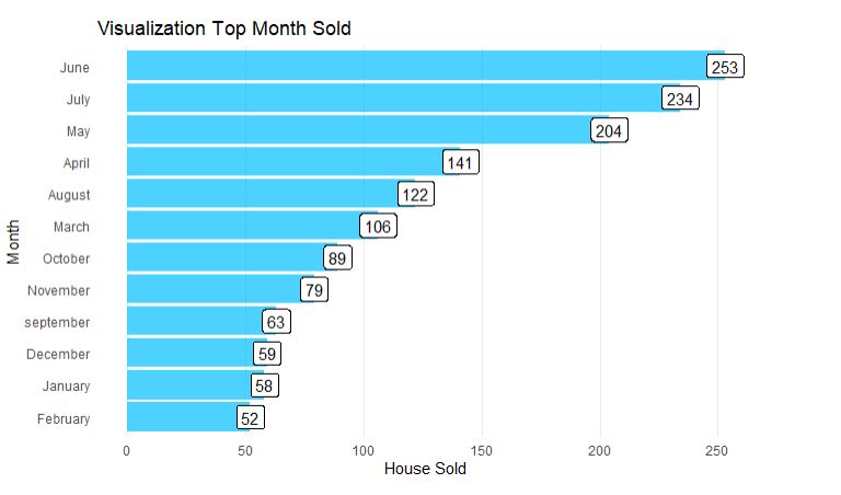
Insight
- The most sold homes are in June, July and May.
- The least sold homes are in February, January and December.
- It can be said that the house sells better in the middle of the year and the worst sales at the beginning and end of the year.
- This can be caused because in the middle of the year a person's financial average can be said to be stable because there is no mid-year holiday or big day in that month.
- While at the beginning of the year, it can be said that people spend a lot of time on holidays or leave because the beginning and end of the year are Christmas and New Year's holidays.
- So that people tend to be reluctant to buy a house when they do a lot of spending, this is what causes the drop in home sales in those months.
- To anticipate this, discounts can be done at the beginning of the year or the end of the year to attract people to buy houses at the end and beginning of the year.