Pima Indians Diabetes

Diabetes is one of the deadliest diseases in the world. It is not only a disease but also creator of different kinds of diseases like heart attack, blindness etc. The normal identifying process is that patients need to visit a diagnostic center, consult their doctor, and sit tight for a day or more to get their reports.
The dataset is originally from the National Institute of Diabetes and Digestive and Kidney Diseases. The objective of the dataset is to diagnostically predict whether or not a patient has diabetes, based on certain diagnostic measurements included in the dataset. Several constraints were placed on the selection of these instances from a larger database. In particular, all patients here are females at least 21 years old of Pima Indian heritage. The datasets consists of several medical predictor variables and one target variable, Outcome. Predictor variables includes the number of pregnancies the patient has had, their BMI, insulin level, age, and so on. We will build a machine learning model to accurately predict whether or not the patients in the dataset have diabetes or not?
Data Fields
Import Package and Data
Started with imports of some basic libraries that are needed throughout the case. This includes Pandas and Numpy for data handling and processing as well as Matplotlib and Seaborn for visualization.
import numpy as np
import pandas as pd
import matplotlib.pyplot as plt
import seaborn as sns
%matplotlib inline

import warnings
warnings.filterwarnings('ignore')

import missingno as msno
For this exercise, the data set (.csv format) is downloaded to a local folder, read into the Jupyter notebook and stored in a Pandas DataFrame.
df = pd.read_csv("C:\My Files\Document\Coding\Datasheet\diabetes.csv")
df.head()
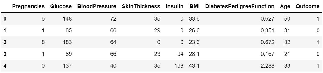
There are some values in Insulin, that cannot be zero. So, need to handle them by imputing.
Descriptive Static of Data
Get statistical information on numerical features.
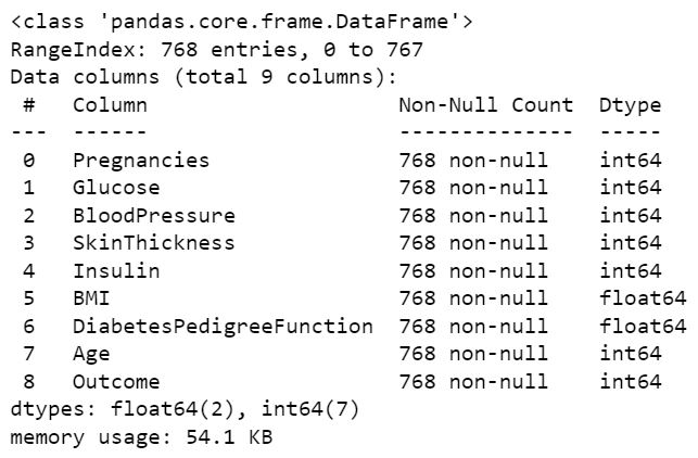
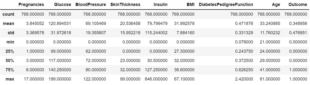
There is a huge variation in mean, and we can see there's no missing values, but for some of the columns like Glucose , BP, Skin Thickness,BMI has 0 as min value, which is not possible, hence we can treat this as missingvalues and impute accordingly.
Handle the Columns with value '0'
Lets check the missing value from the predictor.
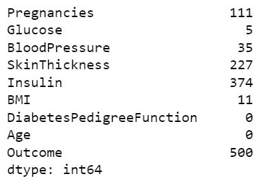
There is so many missing value from the predictor. We cannot drop these values, as our data is very small. So let's handle them by replace it with 0 and mean.
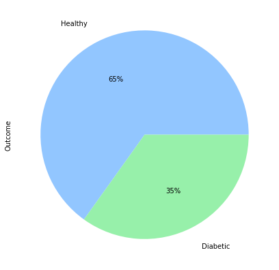
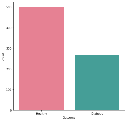
Visualization of Target Variable
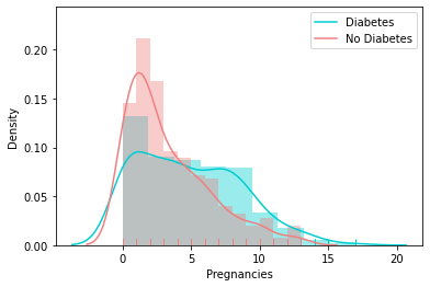
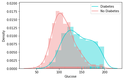
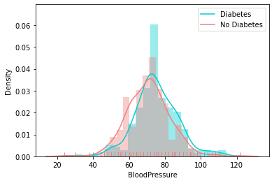
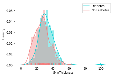
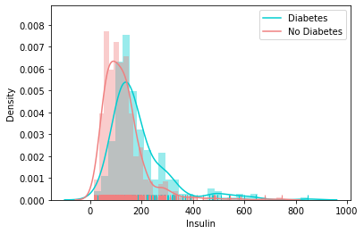
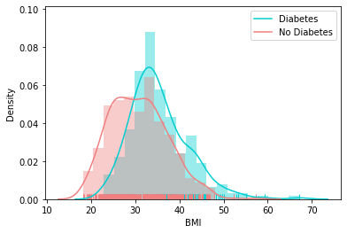
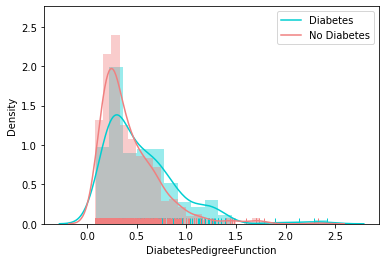
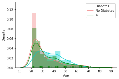
Distribution of Other Feature
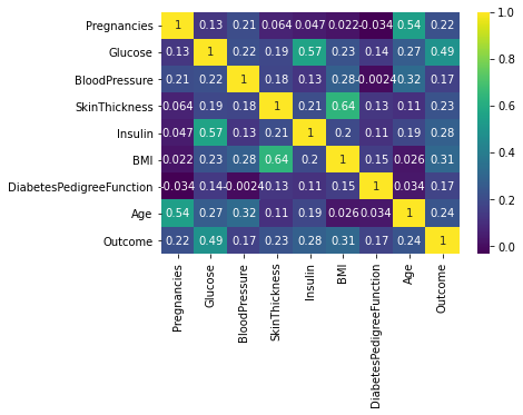
Correlation Matrix
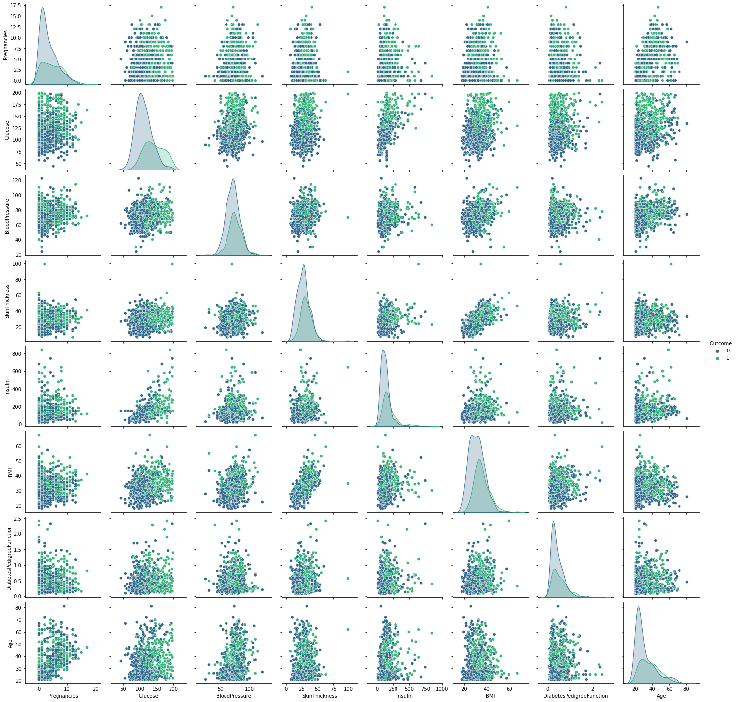
Pair Plot
Machine Learning Model
Split the data into test & train
The train-test split procedure is used to estimate the performance of machine learning algorithms when they are used to make predictions on data not used to train the model.
dx = df.iloc[:, :-1].values
y = df.iloc[:, -1].values
from sklearn.model_selection import train_test_split
x_train, x_test, y_train, y_test = train_test_split(x, y, test_size= 0.2, random_state= 0)
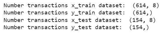
print("Number transactions x_train dataset: ", x_train.shape)
print("Number transactions y_train dataset: ", y_train.shape)
print("Number transactions x_test dataset: ", x_test.shape)
print("Number transactions y_test dataset: ", y_test.shape)
Feature Scaling
Feature Scaling is a technique to standardize the independent features present in the data in a fixed range. It is performed during the data pre-processing to handle highly varying magnitudes or values or units. If feature scaling is not done, then a machine learning algorithm tends to weigh greater values, higher and consider smaller values as the lower values, regardless of the unit of the values.
Standard Scaler: It is a very effective technique which re-scales a feature value so that it has distribution with 0 mean value and variance equals to 1.
dfrom sklearn.preprocessing import StandardScaler
sc = StandardScaler()
x_train = sc.fit_transform(x_train)
x_test = sc.transform(x_test)

from sklearn.metrics import confusion_matrix,classification_report,roc_curve,accuracy_score,auc
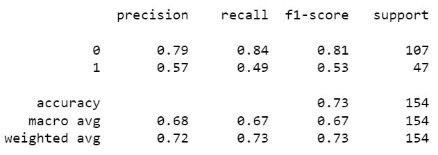
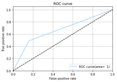
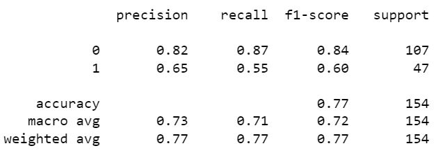
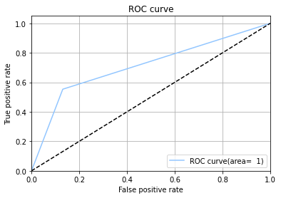
SVM Model
Support Vector Machine or SVM is one of the most popular Supervised Learning algorithms, which is used for Classification as well as Regression problems. However, primarily, it is used for Classification problems in Machine Learning. The goal of the SVM algorithm is to create the best line or decision boundary that can segregate n-dimensional space into classes so that we can easily put the new data point in the correct category in the future. This best decision boundary is called a hyperplane.

Random Forest Model
Random forest classifier creates a set of decision trees from randomly selected subset of training set. It then aggregates the votes from different decision trees to decide the final class of the test object. This works well because a single decision tree may be prone to a noise, but aggregate of many decision trees reduce the effect of noise giving more accurate results.
KNN Model
K-Nearest Neighbour is one of the simplest Machine Learning algorithms based on Supervised Learning technique. It can be used for Regression as well as for Classification but mostly it is used for the Classification problems. K-NN algorithm assumes the similarity between the new case/data and available cases and put the new case into the category that is most similar to the available categories.